Risk management

VaR and Expected Shortfall

Christian Groll

Introduction
Risk measures

Introduction

Definition

risk often is defined as negative deviation of a given target payoff

Convention

risk management is mainly concerned with downsiderisk

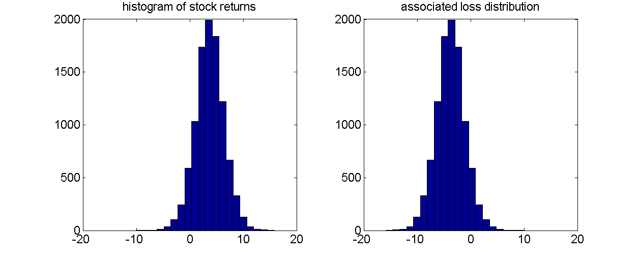
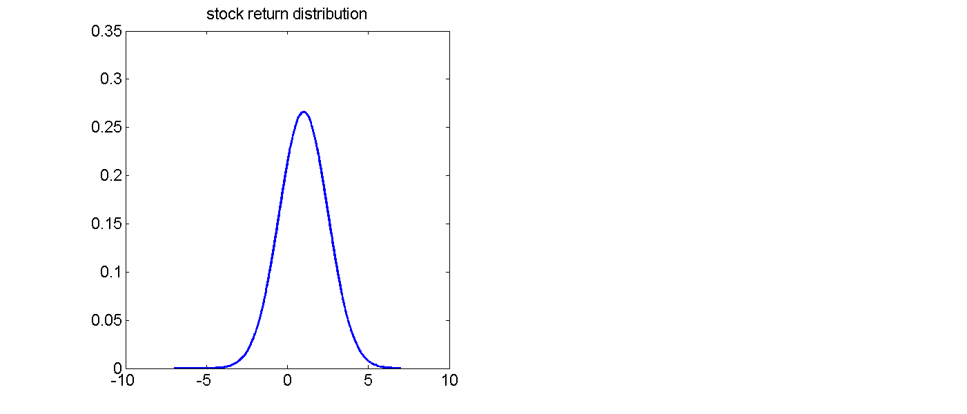
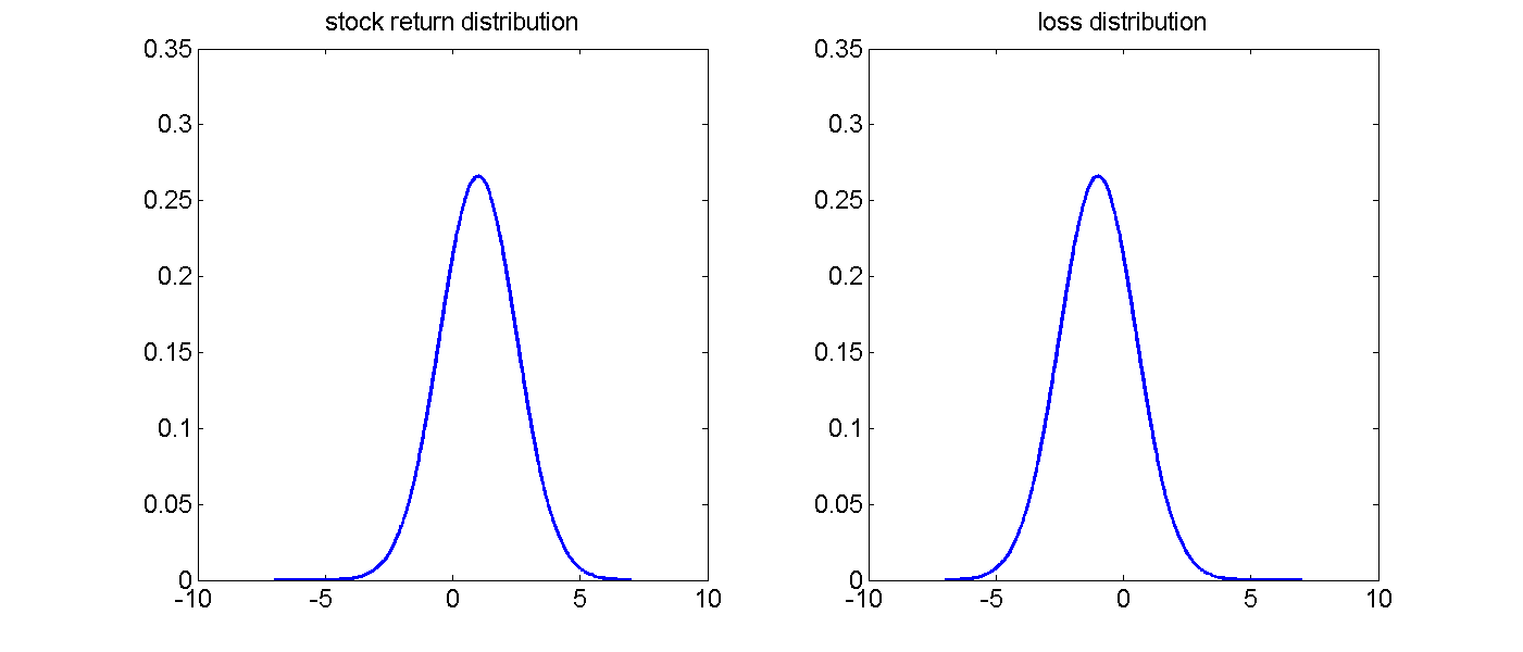
focus on the distribution of losses instead of profits

for prices denoted by P_t , the random variable quantifying losses is given by

$$\begin{equation*} L_{t+1}=-(P_{t+1}-P_{t}) \end{equation*}$$

distribution of losses equals distribution of profits flipped at x-axis

From profits to losses

Quantification of risk

Decisions concerned with managing, mitigating or hedging of risks have to be based on quantification of risk as basis of decision-making:

regulatory purposes: capital buffer proportional to exposure to risk

interior management decisions: freedom of daily traders restricted by capping allowed risk level

corporate management: identification of key risk factors (comparability through risk measures)

Risk measurement frameworks

notional-amount approach

component of standardized approach of Basel capital adequacy framework

nominal value as substitute for outstanding amount at risk

weighting factor representing riskiness of associated asset class as substitute for riskiness of individual asset

advantage: no individual risk assessment necessary - applicable even without empirical data

weakness: diversification benefits and netting unconsidered, strong simplification

scenario analysis

define possible future economic scenarios (stock market crash of -20 percent in major economies, default of Greece government securities,...)

derive associated losses

determine risk as specified quantile of scenario losses (5th largest loss, worst loss, protection against at least 90 percent of scenarios,...)

since scenarios are not accompanied by statements about likelihood of occurrence, probability dimension is completely left unconsidered

scenario analysis can be conducted without any empirical data on the sole grounds of expert knowledge

Quantitative risk management: modeling the loss distribution

incorporates all information about both probability and magnitude of losses

includes diversification and netting effects

usually relies on empirical data

full information of loss distribution reduced to charateristics of distribution for better comprehensibility: risk measures

Types of risk

You are casino owner.

You only have one table of roulette, with one gambler, who plays one game.

He bets 100€ on number 12, and while the odds of winning are 1:36, his payment in case of success will be 3500€ only.

With expected positive payoff, what is your risk of loosing money?

⇒ inherent risk: completely computable

Now assume that you have multiple gamblers per day.

Although you have a pretty good record of the number of gamblers over the last year, you still have to make an estimate about the number of visitors today. What is your risk?

⇒ additional risk due to estimation error

You have been owner of The Mirage Casino in Las Vegas. What was your biggest loss within the last years?

The closing of the show of Siegfried and Roy due to the attack of a tiger led to losses of hundreds of millions of dollars:

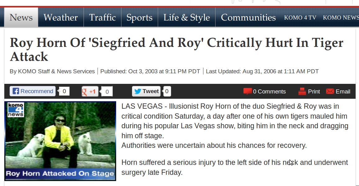
Focusing on gambling losses only left crucial risks outside of the model.

⇒ model risk

Estimation risk vs model risk

Estimation risk:

vanishes with increasing sample size

can be quantified (confidence intervals)

Model risk:

increasing sample size only increases likelihood of detecting wrong model assumptions

For a detailed example illustrating the difference between inherent, estimation and model risk, see this blog post.

Risk measures

Standard deviation

symmetrically capturing positive and negative risks dilutes information about downsiderisk

VaR

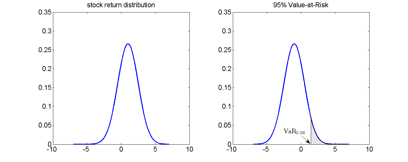
Value-at-Risk (VaR) at confidence level α associated with a given loss distribution L is defined as the smallest value l that is not exceeded with probability higher than (1 − α).

$$\begin{align*} \text{VaR}_{\alpha}&=\inf\{l \in \mathbb{R}: \mathbb{P}(L>l)\leq 1-\alpha\} \\ &=\inf\{l \in \mathbb{R}: F_{L}(l\geq \alpha)\} \end{align*}$$

typical values for α: α = 0.95, α = 0.99 or α = 0.999

as a measure of location, VaR does not provide any information about the nature of losses beyond its value

the losses incurred by investments held on a daily basis exceed the value given by VaR_α only in (1 − α)100 percent of days

with capital buffer equal to VaR_α, financial entity is protected in at least α-percent of days

Illustration

Modeling approaches

In general: underlying loss distribution is not known.

Two modeling approaches VaR:

directly estimate the associated quantile of historical data (historical simulation)

estimate model for underlying loss distribution, and evaluate inverse cdf at required quantile

Involved risks

both approaches entail estimation risk

estimation risk might be of different magnitude

historical simulation does not require any assumptions ⇒ no model risk involved

modeling the loss distribution generally involves distributional assumptions ⇒ model risk due to misspecifications

Mathematical tractability

Derivation of VaR from a model for the loss distribution can be further divided into two situations:

analytical solution for quantile exists

Monte Carlo Simulation when analytic formulas are not available

VaR with normally distributed losses

introductory model: assume normally distributed loss distribution

VaR normal distribution

For given parameters μ_L and σ VaR_α can be calculated analytically by

$$\begin{equation*} \text{VaR}_{\alpha}=\mu_{L}+\sigma\Phi^{-1}(\alpha) \end{equation*}$$

Proof

$$\begin{align*} \mathbb{P}(L\leq VaR_{\alpha})&=\mathbb{P}(L\leq \mu_{L}+\sigma\Phi^{-1}(\alpha))\\ &=\mathbb{P}\left( \frac{L-\mu_{L}}{\sigma} \leq \Phi^{-1}(\alpha)\right) \\ &=\Phi\left( \Phi^{-1}(\alpha) \right) \\ &=\alpha \end{align*}$$

Remarks

note: μ_L in VaR_α = μ_L + σΦ^− 1(α) is the expectation of the loss distribution

if μ denotes the expectation of the asset return, i.e. the expectation of the profit, then the formula has to be modified to

$$\begin{equation*} VaR_{\alpha}=-\mu+\sigma\Phi^{-1}(\alpha) \end{equation*}$$

Model risk

In practice, the assumption of normally distributed returns usually can be rejected both for loss distributions associated with credit and operational risk, as well as for loss distributions associated with market risk at high levels of confidence.

Expected Shortfall

Expected Shortfall

The Expected Shortfall (ES) with confidence level α denotes the conditional expected loss, given that the realized loss is equal to or exceeds the corresponding value of VaR_α:

$$\begin{equation*} \text{ES}_{\alpha}=\mathbb{E}[L \vert L \geq \text{VaR}_{\alpha}] \end{equation*}$$

Interpretation: given that we are in one of the (1 − α)100 percent worst periods, how high is the loss that we have to expect?

Expected Shortfall as expectation of conditional loss distribution:

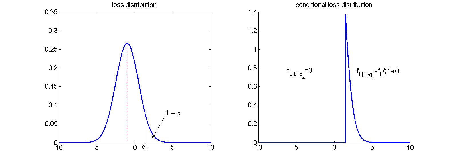
ES contains information about nature of losses beyond VaR:

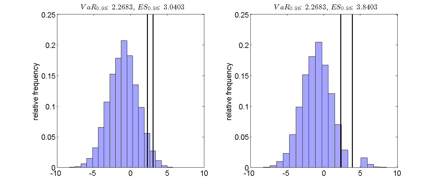
Modeling approaches

Again, there are two approaches to derive ES:

directly estimate the mean of all values greater than the associated quantile of historical data
estimate model for underlying loss distribution, and calculate expectation of conditional loss distribution

Both approaches come with the same risks as for the case of VaR.

ES with normally distributed losses

ES normal distribution

Given that L ∼ 𝒩(μ_L, σ²), the Expected Shortfall of L is given by

$$\begin{equation*} \text{ES}_{\alpha}=\mu_{L}+\sigma \frac{\phi\left( \Phi^{-1}(\alpha) \right) }{1-\alpha} \end{equation*}$$

Proof:

$$\begin{align*} ES_{\alpha} & =\mathbb{E}\left[L|L\geq VaR_{\alpha}\right]\\ & =\mathbb{E}\left[L|L\geq\mu_{L}+\sigma\Phi^{-1}\left(\alpha\right)\right]\\ & =\mathbb{E}\left[L|\frac{L-\mu_{L}}{\sigma}\geq\Phi^{-1}\left(\alpha\right)\right]\\ & =\mu_{L}-\mu_{L}+\mathbb{E}\left[L|\frac{L-\mu_{L}}{\sigma}\geq\Phi^{-1}\left(\alpha\right)\right]\\ & =\mu_{L}+\mathbb{E}\left[L-\mu_{L}|\frac{L-\mu_{L}}{\sigma}\geq\Phi^{-1}\left(\alpha\right)\right]\\ & =\mu_{L}+\sigma\mathbb{E}\left[\frac{L-\mu_{L}}{\sigma}|\frac{L-\mu_{L}}{\sigma}\geq\Phi^{-1}\left(\alpha\right)\right]\\ & =\mu_{L}+\sigma\mathbb{E}\left[Y|Y\geq\Phi^{-1}\left(\alpha\right)\right],\,\mbox{ with }Y\sim\mathcal{N}\left(0,1\right) \end{align*}$$

Furthermore, for ℙ(Y ≥ Φ^− 1(α)) we get:

$$\begin{equation*} \mathbb{P}\left(Y\geq\Phi^{-1}\left(\alpha\right)\right)=1-\mathbb{P}\left(Y\leq\Phi^{-1}\left(\alpha\right)\right)=1-\Phi\left(\Phi^{-1}\left(\alpha\right)\right)=1-\alpha, \end{equation*}$$

so that we get as conditional density ϕ_{Y|Y ≥ Φ^− 1(α)}(y):

$$\begin{align*} \phi_{Y|Y\geq\Phi^{-1}\left(\alpha\right)}\left(y\right) & =\frac{\phi\left(y\right)\mathbf{1}_{\left\{ y\geq\Phi^{-1}\left(\alpha\right)\right\} }}{\mathbb{P}\left(Y\geq\Phi^{-1}\left(\alpha\right)\right)}\\ & =\frac{\phi\left(y\right)\mathbf{1}_{\left\{ y\geq\Phi^{-1}\left(\alpha\right)\right\} }}{1-\alpha}. \end{align*}$$

Hence, the integral can be calculated as

$$\begin{align*} \mathbb{E}\left[Y|Y\geq\Phi^{-1}\left(\alpha\right)\right] & =\int_{-\infty}^{\infty}y\cdot\phi_{Y|Y\geq\Phi^{-1}\left(\alpha\right)}\left(y\right)dy\\ & =\int_{\Phi^{-1}\left(\alpha\right)}^{\infty}y\cdot\frac{\phi\left(y\right)}{1-\alpha}dy\\ & =\frac{1}{1-\alpha}\int_{\Phi^{-1}\left(\alpha\right)}^{\infty}y\cdot\phi\left(y\right)dy\\ & \overset{\left(\star\right)}{=}\frac{1}{1-\alpha}\left[-\phi\left(y\right)\right]_{\Phi^{-1}\left(\alpha\right)}^{\infty}\\ & =\frac{1}{1-\alpha}\left(0+\phi\left(\Phi^{-1}\left(\alpha\right)\right)\right)\\ & =\frac{\phi\left(\Phi^{-1}\left(\alpha\right)\right)}{1-\alpha}, \end{align*}$$

with ( ⋆ ):

$$\begin{equation*} \left(-\phi\left(y\right)\right)^{'}=-\frac{1}{\sqrt{2\pi}}\exp\left(-\frac{y^{2}}{2}\right)\cdot\left(-\frac{2y}{2}\right)=y\cdot\phi\left(y\right) \end{equation*}$$

Exercise

Example: Meaning of VaR

You have invested in an investment fonds of size 500,000 €. The manager of the fonds tells you that the 99% Value-at-Risk for a time horizon of one year amounts to 5% of the portfolio value. Explain the information conveyed by this statement.

Solution

for continuous loss distribution we have equality
$$\begin{equation*} \mathbb{P}\left(L\geq \text{VaR}_{\alpha}\right)=1-\alpha \end{equation*}$$

transform relative statement about losses into absolute quantity

$$\begin{equation*} \text{VaR}_{\alpha}=0.05\cdot500,000=25,000 \end{equation*}$$

pluggin into formula leads to

$$\begin{equation*} \mathbb{P}\left(L\geq25,000\right)=0.01 \end{equation*}$$

Interpretation:

"with probability 1% you will lose 25,000 € or more"

a capital cushion of height VaR_0.99 = 25000 is sufficient in exactly 99% of the times for continuous distributions

Example: discrete case

exemplary discrete loss distribution:

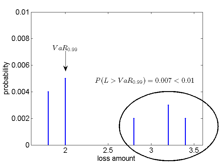
the capital cushion provided by VaR_α would be sufficient in even 99.3% of the times

interpretation of statement: "with probability of maximal 1% you will lose 25,000 € or more"

Example: Meaning of ES

The fondsmanager corrects himself. Instead of the Value-at-Risk, it is the Expected Shortfall that amounts to 5% of the portfolio value. How does this statement have to be interpreted? Which of both cases does imply the riskier portfolio?

Interpretation

given that one of the 1% worst years occurs, the expected loss in this year will amount to 25,000 €

Due to

$$\begin{equation*} \text{VaR}_{\alpha}\leq \text{ES}_{\alpha} \end{equation*}$$

the first statement implies:

$$\begin{equation*} \text{ES}_{\alpha}\geq25,000€ \end{equation*}$$

⇒ the first statement implies the riskier portfolio

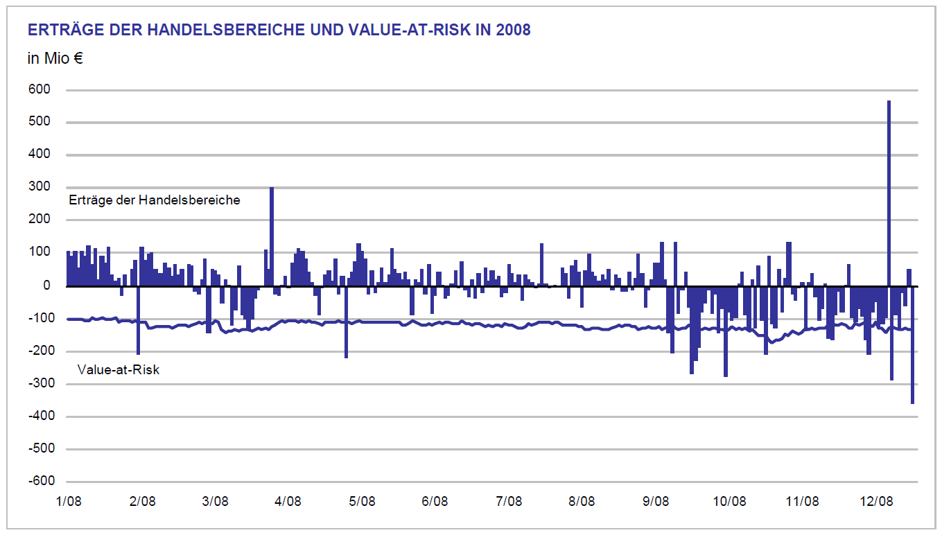
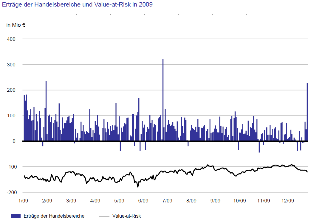
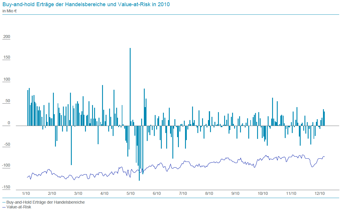
Real world: model risk

besides sophisticated modeling approaches even Deutsche Bank seems to fail at VaR-estimation: VaR_0.99

Backtesting

How good did estimated VaR values perform in-sample?

compare exceedance / hit rate with desired confidence level

$$\begin{equation*} \frac{1}{N}\sum_{i=1}^{N}\mathbf{1}_{\{L_{i}>\text{VaR}\}}\overset{?}{=}\alpha \end{equation*}$$