Risk management
Introduction to the modeling of assets
Christian Groll
Interest rates and returns
General problem
Quantity of interest
$$\begin{equation*} \bf{Z}=g(\bf{X}),\quad \bf{X}=(X_{1},\ldots, X_{d}) \end{equation*}$$
- Xi are random variables
- Xi represent uncertain risk factors
Examples
portfolio return
- individual stocks (X1, …, Xd)
- g is aggregation function
option payoff
- single underlying X1
- g is payoff function
Difference to regression setting
- Xi part of the model:
- in regression analysis, all Xi are taken as given
- here we need to specify a distribution for (X1, …, Xd)
Justification
- in regression analysis, explanatory variables with influence on first moment are observable upfront
- for financial variables, explanatory variables (X1, …, Xd) sometimes only become observable simultaneously to Z
- many financial variables tend to exhibit almost constant mean over time: how they are distributed around their mean is important
Certain future payments
- in the simplest case, all risk factors (X1, …, Xd) are perfectly known
Example
- bank account with given interest rate
Aggregation
- even without uncertainty, our quantity of interest commonly implies a multi-dimensional setting
Example
- multi-period wealth calculation with given annual interest rates
Interest and compounding
given an interest rate of r per period and initial wealth Wt, the wealth one period ahead is calculated as
$$\begin{equation*} W_{t+1}=W_{t}\left(1+r\right) \end{equation*}$$
Example
- r = 0.05 (annual rate), W0 = 500.000, after one year
$$500.000\left(1+\frac{5}{100}\right)= 500.000\left(1+0.05\right)=525.000$$
- multi-period compound interest:
$$\begin{equation*} W_{T}(r,W_{0})=W_{0}(1+r)^{T} \end{equation*}$$
Non-constant interest rates
- for the case of changing annual interest rates, end-of-period wealth is given by
$$\begin{align*} W_{1:t} & =\left(1+r_{0}\right)\cdot\left(1+r_{1}\right)\cdot...\cdot\left(1+r_{t-1}\right)\\ & =\prod_{i=0}^{t-1}\left(1+r_{i}\right) \end{align*}$$
Logarithmic interest rates
- logarithmic interest rates or continuously compounded interest rates are given by
$$\begin{equation*} r_{t}^{log}:=\ln\left(1+r_{t}\right) \end{equation*}$$
Aggregation
- with logarithmic interest rates aggregation becomes a sum rather than a product of sub-period interest rates:
$$\begin{align*} r_{1:t}^{log}&=\ln\left( 1+r_{1:t} \right) \\ &=\ln\left(\prod_{i=1}^{t}\left(1+r_{i}\right)\right) \\ &=\ln\left(1+r_{1}\right)+\ln\left(1+r_{2}\right)+\ldots+\ln\left(1+r_{t}\right)\\ & =r_{1}^{log}+r_{2}^{log}+\ldots+r_{t}^{log}\\ &=\sum_{i=1}^{t} r_{i}^{log} \end{align*}$$
Compounding at higher frequency
- compounding can occur more frequently than at annual intervals
- m times per year: Wm, t(r) denotes wealth in t for W0 = 1
Biannually
after six months:
$$\begin{equation*} W_{2,\frac{1}{2}}(r)=\left(1+\frac{r}{2}\right) \end{equation*}$$
Effective annual rate
- the effective annual rate Reff is defined as the wealth after one year, given an initial wealth W0 = 1
- with biannual compounding, we get
$$\begin{equation*} R^{eff}:=W_{2,1}(r)=\left(1+\frac{r}{2}\right)\left(1+\frac{r}{2}\right)=\left(1+\frac{r}{2}\right)^{2} \end{equation*}$$
- it exceeds the simple annual rate:
$$\begin{equation*} \left(1+\frac{r}{2}\right)^{2}>\left(1+r\right)\Rightarrow W_{2,1}\left(r\right)>W_{1,1}\left(r\right) \end{equation*}$$
m interest payments within a year
- effective annual rate after one year:
$$\begin{equation*} R^{eff}=W_{m,1}(r)=\left(1+\frac{r}{m}\right)^{m} \end{equation*}$$
- for wealth after T years we get:
$$\begin{equation*} W_{m,T}(r)=\left(1+\frac{r}{m}\right)^{mT} \end{equation*}$$
wealth is an increasing function of the interest payment frequency:
$$\begin{equation*} W_{m_{1},t}\left(r\right)>W_{m_{2},t}\left(r\right),\,\forall t\,\mbox{and}\, m_{1}>m_{2} \end{equation*}$$
Continuous compounding
the continuously compounded rate is given by the limit
$$\begin{equation*} W_{\infty,1}\left(r\right)=\lim_{m\rightarrow\infty}\left(1+\frac{r}{m}\right)^{m}=e^{r} \end{equation*}$$
compounding over T periods leads to
$$\begin{equation*} W_{\infty,T}\left(r\right)=\lim_{m\rightarrow\infty}\left(1+\frac{r}{m}\right)^{mT}=\left(\lim_{m\rightarrow\infty}\left(1+\frac{r}{m}\right)^{m}\right)^{T}=e^{rT} \end{equation*}$$
- under continuous compounding the value of an initial investment of W0 grows exponentially fast
- comparatively simple for calculation of interest accrued in between dates of interest payments
| T | m = 1 | m = 2 | m = 3 | ∞ |
|---|---|---|---|---|
| 1 | 1030 | 1030.2 | 1030.3 | 1030.5 |
| 2 | 1060.9 | 1061.4 | 1061.6 | 1061.8 |
| 3 | 1092.7 | 1093.4 | 1093.8 | 1094.2 |
| 5 | 1159.3 | 1160.5 | 1161.2 | 1161.8 |
| ⋯ | ⋯ | ⋯ | ||
| 9 | 1304.8 | 1307.3 | 1308.6 | 1310 |
| 10 | 1343.9 | 1346.9 | 1348.3 | 1349.9 |
Development of initial investment W0 = 1000 over 10 years, subject to different interest rate frequencies, with annual interest rate r = 0.03
Effective logarithmic rates
For logarithmic interest rates, a higher compounding frequency leads to
$$\begin{align*} r^{log; eff}&=\ln(R^{eff})\\ &=\ln(W_{m,1})\\ &=\ln\left( \left(1 + \frac{r}{m}\right)^{m} \right)\\ &\overset{m\rightarrow\infty}{\rightarrow}\ln(\exp{(r)})\\ &=r \end{align*}$$
Interpretation: If the bank were compounding interest rates continuously, the nominal interest rate r would equal the logarithmic effective rate.
Also:
- if rlog; eff = r for continuous compounding,
- and continuous compounding leads to almost identical end of period wealth as simple compounding (see table above)
- the logarithmic transformation rlog = ln(1 + r) does change the value only marginally: rlog ≈ r
Conclusion
In other words:
- we can interpret log-interest rates as roughly equal to simple rates
- still, log-interest rates are better to work with, as they increase linearly through aggregation over time
Conclusion
But: if interest rates get bigger, the approximation of simple compounding by continuous compounding gets worse!
- ln(1 + x) = x for x = 0
- ln(1 + x) ≈ x for x ≠ 0
Prices and returns
Returns on speculative assets
- while interest rates of fixed-income assets are usually known prior to the investment, returns of speculative assets have to be calculated after observation of prices
- returns on speculative assets usually vary from period to period
- let Pt denote the price of a speculative asset at time t
net return during period t:
$$\begin{equation*} r_{t}:=\frac{P_{t}-P_{t-1}}{P_{t-1}}=\frac{P_{t}}{P_{t-1}}-1 \end{equation*}$$
gross return during period t:
$$\begin{equation*} R_{t}:=(1+r_{t})=\frac{P_{t}}{P_{t-1}} \end{equation*}$$
- returns calculated this way are called discrete returns
Continuously compounded returns
- defining the log return, or continuously compounded return, by
$$\begin{equation*} r_{t}^{log}:=\ln R_{t}=\ln\left(1+r_{t}\right)=\ln\frac{P_{t}}{P_{t-1}}=\ln P_{t}-\ln P_{t-1} \end{equation*}$$
Exercise
Investor A and investor B both made one investment each. While investor A was able to increase his investment sum of 100 to 140 within 3 years, investor B increased his initial wealth of 230 to 340 within 5 years. Which investor did perform better?
Exercise: solution
- calculate mean annual interest rate for both investors
investor A :
$$\begin{align*} P_{T} & =P_{0}\left(1+r\right)^{T} & \Leftrightarrow\\ 140 & =100\left(1+r\right)^{3} & \Leftrightarrow\\ \sqrt[3]{\frac{140}{100}} & =\left(1+r\right) & \Leftrightarrow\\ r_{A} & =0.1187 \end{align*}$$
investor B :
$$\begin{equation*} r_{B}=\left(\sqrt[5]{\frac{340}{230}}-1\right)=0.0813 \end{equation*}$$hence, investor A has achieved a higher return on his investment
Using continuous returns
- for comparison, using continuous returns
Continuous case
- continuously compounded returns associated with an evolution of prices over a longer time period is given by
$$\begin{equation*} P_{T}=P_{0}e^{rT}\Leftrightarrow\frac{P_{T}}{P_{0}}=e^{rT}\Leftrightarrow\ln\left(\frac{P_{T}}{P_{0}}\right)=\ln\left(e^{rT}\right)=rT \end{equation*}$$
$$\begin{equation*} r=\frac{\left(\ln P_{T}-\ln P_{0}\right)}{T} \end{equation*}$$
Continuous case
plugging in leads to
$$\begin{equation*} r_{A}=\frac{\left(\ln140-\ln100\right)}{3}=0.1122 \end{equation*}$$
$$\begin{equation*} r_{B}=\frac{\left(\ln340-\ln230\right)}{5}=0.0782 \end{equation*}$$
- conclusion: while the case of discrete returns involves calculation of the n-th root, the continuous case is computationally less demanding
- while continuous returns differ from their discrete counterparts, the ordering of both investors is unchanged
- keep in mind: so far we only treat returns retrospectively, that is, with given and known realization of prices, where any uncertainty involved in asset price evolutions already has been resolved
Comparing different investments
comparison of returns of alternative investment opportunities over different investment horizons requires computation of an average gross return $\bar{R}$ for each investment, fulfilling:
$$\begin{equation*} P_{t}\bar{R}^{n}\overset{!}{=}P_{t}R_{t}\cdot\ldots\cdot R_{t+n-1}=P_{t+n} \end{equation*}$$
- in net returns:
$$\begin{equation*} P_{t}\left(1+\bar{r}\right)^{n}\overset{!}{=}P_{t}\left(1+r_{t}\right)\cdot\ldots\cdot\left(1+r_{t+n-1}\right) \end{equation*}$$
- solving for $\bar{r}$ leads to
$$\begin{equation*} \bar{r}=\left(\prod_{i=0}^{n-1}\left(1+r_{t+i}\right)\right)^{1/n}-1 \end{equation*}$$
- the annualized gross return is not an arithmetic mean, but a geometric mean
Example
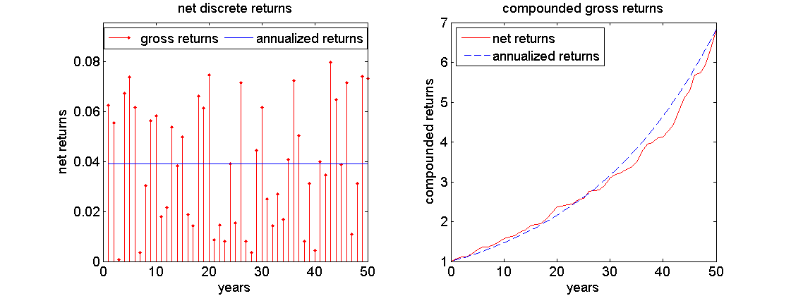
Left: randomly generated returns between 0 and 8 percent, plotted against annualized net return rate. Right: comparison of associated compound interest rates.
The annualized return of 1.0392 is unequal to the simple arithmetic mean over the randomly generated interest rates of 1.0395!
Example
- two ways to calculate annualized net returns for previously generated random returns:
Direct way
using gross returns, taking 50-th root:
$$\begin{align*} \bar{r}_{t,t+n-1}^{ann} & =\left(\prod_{i=0}^{n-1}\left(1+r_{t+i}\right)\right)^{1/n}-1\\ & =\left(1.0626\cdot1.0555\cdot...\cdot1.0734\right)^{1/50}-1\\ & =\left(6.8269\right)^{1/50}-1\\ & =0.0391 \end{align*}$$
Via log returns
transfer the problem to the logarithmic world:
- convert gross returns to log returns:
$$\begin{equation*} \left[1.0626,1.0555,\ldots,1.0734\right]\overset{log}{\longrightarrow}\left[0.0607,0.0540,\ldots,0.0708\right] \end{equation*}$$
- use arithmetic mean to calculate annualized return in the logarithmic world:
$$\begin{align*} r_{t,t+n-1}^{log}=\sum_{i=0}^{n-1}r_{t+i}^{log}&=\left(0.0607+0.0540+...+0.0708\right)=1.9226\\ \bar{r}_{t,t+n-1}^{log}&=\frac{1}{n}r_{t,t+n-1}^{log}=\frac{1}{50}1.9226=0.0385 \end{align*}$$
Example
- convert result back to normal world:
$$\begin{equation*} \bar{r}_{t,t+n-1}^{ann}=e^{\bar{r}_{t,t+n-1}^{log}}-1=e^{0.0385}-1=0.0391 \end{equation*}$$
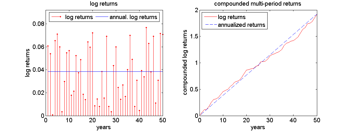
Summary
multi-period gross returns result from multiplication of one-period returns: hence, exponentially increasing
multi-period logarithmic returns result from summation of one-period returns: hence, linearly increasing
different calculation of returns from given portfolio values:
$$\begin{equation*} r_{t}=\frac{P_{t}-P_{t-1}}{P_{t}}\quad\quad r_{t}^{log}=\ln\left(\frac{P_{t}}{P_{t-1}}\right)=\ln P_{t}-\ln P_{t-1} \end{equation*}$$
However, because of
$$\begin{equation*} \ln\left(1+x\right)\approx x \end{equation*}$$
discrete net returns and log returns are approximately equal:
$$\begin{equation*} r_{t}^{log}=\ln\left(R_{t}\right)=\ln\left(1+r_{t}\right)\approx r_{t} \end{equation*}$$
- given that prices / returns are already known, with no uncertainty left, continuous returns are computationally more efficient
- discrete returns can be calculated via a detour to continuous returns
- as the transformation of discrete to continuous returns does not change the ordering of investments, and as logarithmic returns are still interpretable since they are the limiting case of discrete compounding, why shouldn't we just stick with continuous returns overall?
- however: the main advantage only crops up in a setting of uncertain future returns, and their modelling as random variables!
Importance of returns
Why are asset returns so pervasive if asset prices are the real quantity of interest in many cases?
Non-stationarity
Most prices are not stationary:
- over long horizons stocks tend to exhibit a positive trend
- distribution changes over time
Consequence
- historic prices are not representative for future prices: mean past prices are a bad forecast for future prices
Returns
- returns are stationary in most cases
⇒ historic data can be used to estimate their current distribution
General problem
Quantity of interest
$$\begin{equation*} \bf{Z}=g(\bf{X}),\quad \bf{X}=(X_{1},\ldots, X_{d}) \end{equation*}$$
- as statistical requirements tend to force us to use returns instead of prices, almost always at least some Xi represent returns
Time horizon and aggregation
- lower frequency returns can be expressed as aggregation of higher frequency returns
- lack of data for lower frequency returns (as they need to be non-overlapping)
⇒ long horizons usually require aggregation of higher frequency returns: Xt, Xt + 1, …
Outlook: mathematical tractability
Only with log-returns we preserve a chance to end up with a linear function:
Quantity of interest
$$\begin{align*} \bf{Z}&=g(\bf{X})\\ &=g(Y_{t}, Y_{t+1}, \ldots, X_{i}) \\ &=\hat{g}(Y_{t} + Y_{t+1} + \ldots, X_{i}) \end{align*}$$
Outlook: statistical fitting
The central limit theorem could justify modelling logarithmic returns as normally distributed:
- returns can be decomposed into summation over returns of higher frequency: e.g. annual returns are the sum of 12 monthly returns, 52 weakly returns, 365 daily returns,...
The central limit theorem states:
Independent of the distribution of high frequency returns, any sum of them follows a normal distribution, provided that the sum involves sufficiently many summands, and the following requirements are fulfilled:
- the high frequency returns are independent of each other
- the distribution of the low frequency returns allows finite second moments (variance)
- this reasoning does not apply to net / gross returns, since they can not be decomposed into a sum of lower frequency returns
- keep in mind: these are only hypothetical considerations, since we have not seen any real world data so far!
Probability theory
- randomness: the result is not known in advance
- probability theory: captures randomness in mathematical framework
Probability spaces and random variables
- sample space Ω: set of all possible outcomes or elementary events ω
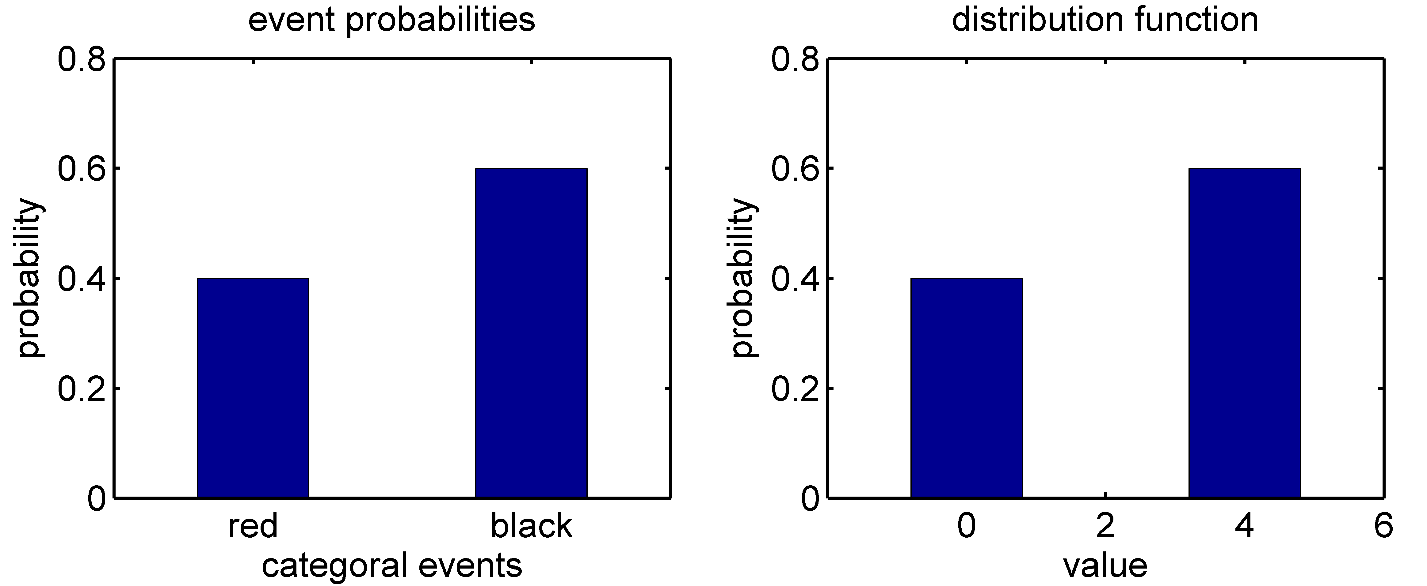
Examples: discrete sample space:
- roulette: Ω1 = {red, black}
- performance: Ω2 = {good, moderate, bad}
- die: Ω3 = {1, 2, 3, 4, 5, 6}
Examples: continuous sample space:
- temperature: Ω4 = [ − 40, 50]
- log-returns: Ω5 = ] − ∞, ∞[
Events
- a subset A ⊂ Ω consisting of more than one elementary event ω is called event
Examples
- "at least moderate performance":
$$\begin{equation*} A=\left\{ \mbox{good,moderate}\right\} \subset\Omega_{2} \end{equation*}$$
- "even number":
$$\begin{equation*} A=\left\{ 2,4,6\right\} \subset\Omega_{3} \end{equation*}$$
- "warmer than 10 degrees":
$$\begin{equation*} A=]10,\infty[\subset\Omega_{4} \end{equation*}$$
Event space
- the set of all events of Ω is called event space ℱ
- usually it contains all possible subsets of Ω: it is the power set of 𝒫(Ω)
Events
- {} denotes the empty set
Event space example
$$\begin{align*} \mathcal{P}\left(\Omega_{2}\right)&=\left\{ \Omega,\left\{ \right\} \right\} \cup\left\{ \mbox{good}\right\} \cup\left\{ \mbox{moderate}\right\} \\ &=\cup\left\{ \mbox{bad}\right\} \cup\left\{ \mbox{good,moderate}\right\} \cup\left\{ \mbox{good,bad}\right\} \cup\left\{ \mbox{moderate,bad}\right\} \end{align*}$$
Events
- an event A is said to occur if any ω ∈ A occurs
Example
If the performance happens to be ω = {good}, then also the event A = "at least moderate performance" has occured, since ω ⊂ A.
Probability measure
A real-valued set function ℙ : ℱ → ℝ, with properties
- ℙ(A) > 0 for all A ⊆ Ω
- ℙ(Ω) = 1
- For each finite or countably infinite collection of disjoint events (Ai) it holds:
ℙ( ∪ i ∈ IAi) = ∑i ∈ Iℙ(Ai)
⇒ quantifies for each event a probability of occurance
Definition
The 3-tuple {Ω, ℱ, ℙ} is called probability space.
Random variable
- instead of outcome ω itself, usually a mapping or function of ω is in the focus: when playing roulette, instead of outcome "red" it is more useful to consider associated gain or loss of a bet on "color"
- conversion of categoral outcomes to real numbers allows for further measurements / information extraction: expectation, dispersion,...
Definition
Let {Ω, ℱ, ℙ} be a probability space. If X : Ω → ℝ is a real-valued function with the elements of Ω as its domain, then X is called random variable.
Example
Density function
- a discrete random variable consists of a countable number of elements, while a continuous random variable can take any real value in a given interval
- a probability density function determines the probability (possibly 0) for each event
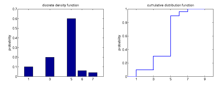
Discrete density function
For each xi ∈ X(Ω) = {xi|xi = X(ω), ω ∈ Ω}, the function
$$\begin{equation*} f\left(x_{i}\right)=\mathbb{P}\left(X=x_{i}\right) \end{equation*}$$
assigns a value corresponding to the probability.
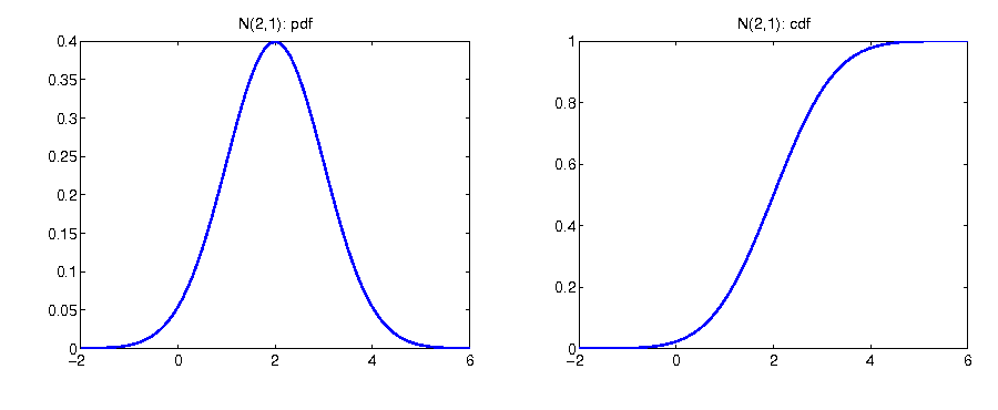
Continuous density function
In contrast, the values of a continuous density function f(x), x ∈ {x|x = X(ω), ω ∈ Ω} are not probabilities itself. However, they shed light on the relative probabilities of occurrence. Given f(y) = 2 ⋅ f(z), the occurrence of y is twice as probable as the occurrence of z.
Example
Cumulative distribution function The cumulative distribution function (cdf) of random variable X, denoted by F(x),
indicates the probability that X takes on a value that is lower than or equal to x, where x is any real number. That is
$$\begin{equation*} F\left(x\right)=\mathbb{P}\left(X\leq x\right),\quad-\infty<x<\infty. \end{equation*}$$
a cdf has the following properties:
- F(x) is a nondecreasing function of x;
- limx → ∞F(x) = 1;
- limx → − ∞F(x) = 0.
- furthermore:
$$\begin{equation*} \mathbb{P}\left(a<X\leq b\right)=F\left(b\right)-F\left(a\right),\quad\mbox{for all }b>a \end{equation*}$$
Interrelation pdf and cdf: discrete case
$$\begin{equation*} F\left(x\right)=\mathbb{P}\left(X\leq x\right)=\sum_{x_{i}\leq x}\mathbb{P}\left(X=x_{i}\right) \end{equation*}$$
Interrelation pdf and cdf: continuous case
$$\begin{equation*} F\left(x\right)=\mathbb{P}\left(X\leq x\right)=\int_{-\infty}^{x}f\left(u\right)du \end{equation*}$$
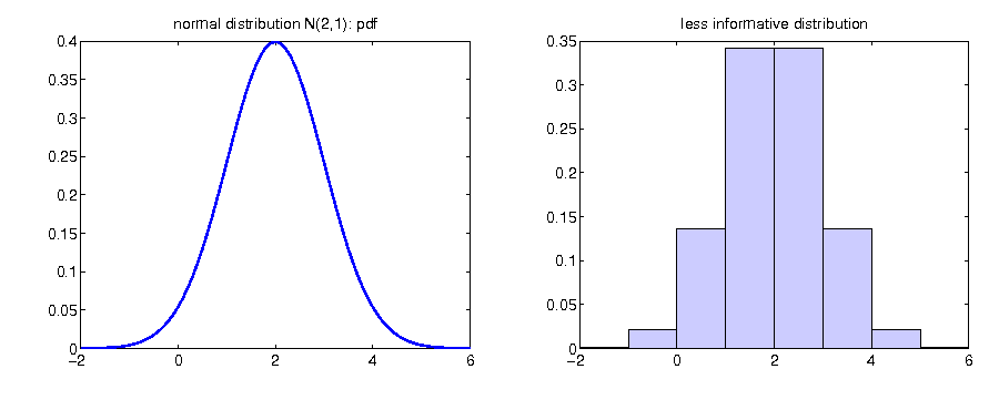
Information reduction
Modeling information
- both cdf as well as pdf, which is the derivative of the cdf, provide complete information about the distribution of the random variable
- may not always be necessary / possible to have complete distribution
- incomplete information modelled via event space ℱ
Example
- sample space given by Ω = {1, 3, 5, 6, 7}
modeling complete information about possible realizations:
$$\begin{align*} \mathcal{P}\left(\Omega\right) & =\left\{ 1\right\} \cup\left\{ 3\right\} \cup\left\{ 5\right\} \cup\left\{ 6\right\} \cup\left\{ 7\right\} \cup\\ & \cup\left\{ 1,3\right\} \cup\left\{ 1,5\right\} \cup...\cup\left\{ 6,7\right\} \cup\left\{ 1,3,5\right\} \cup...\cup\left\{ 5,6,7\right\} \cup\\ & \cup\left\{ 1,3,5,6\right\} \cup...\cup\left\{ 3,5,6,7\right\} \cup\left\{ \Omega,\left\{ \right\} \right\} \end{align*}$$
example of event space representing incomplete information could be
$$\begin{equation*} \mathcal{F}=\left\{ \left\{ 1,3\right\} ,\left\{ 5\right\} ,\left\{ 6,7\right\} \right\} \cup\left\{ \left\{ 1,3,5\right\} ,\left\{ 1,3,6,7\right\} ,\left\{ 5,6,7\right\} \right\} \cup\left\{ \Omega,\left\{ \right\} \right\} \end{equation*}$$
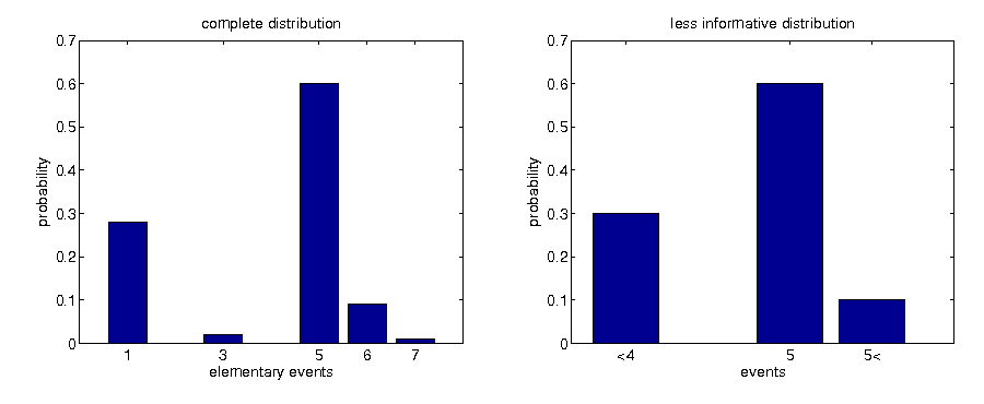
- given only incomplete information, originally distinct distributions can become indistinguishable
Information reduction discrete
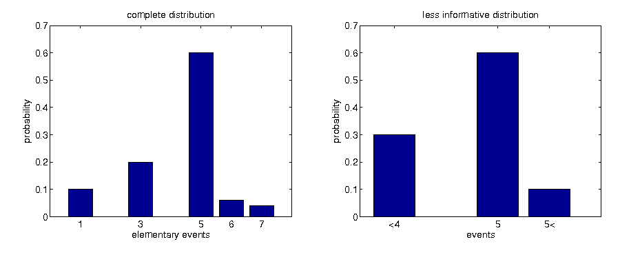
Information reduction discrete
Information reduction continuous
Measures of random variables
- complete distribution may not always be necessary
- compress information of complete distribution for better comparability with other distributions
- compressed information is easier to interpret
- example: knowing "central location" together with an idea by how much X may fluctuate around the center may be sufficient
Classification with respect to several measures can be sufficient:
- probability of negative / positive return
- return on average
- worst case
- measures of location and dispersion
Given only incomplete information conveyed by measures, distinct distributions can become indistinguishable.
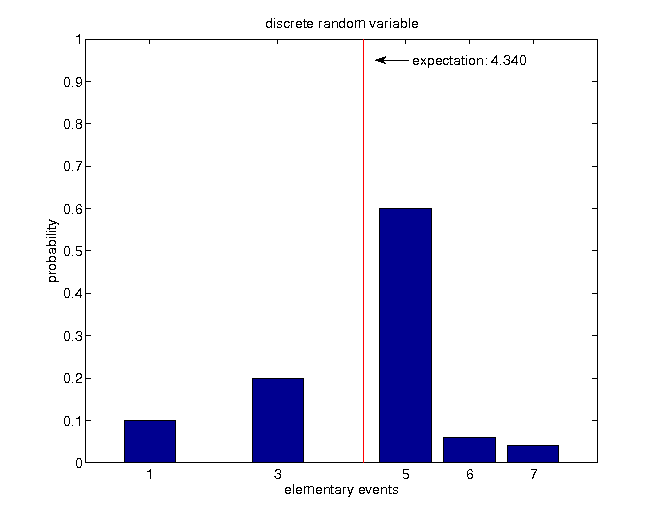
Expectation
The expectation, or mean, is defined as a weighted average of all possible realizations of a random variable.
Discrete random variables
The expected value 𝔼[X] is defined as
$$\begin{equation*} \mathbb{E}\left[X\right]=\mu_{X}=\sum_{i=1}^{N}x_{i}\mathbb{P}\left(X=x_{i}\right). \end{equation*}$$
Continuous random variables
For a continuous random variable with density function f(x) :
$$\begin{equation*} \mathbb{E}\left[X\right]=\mu_{X}=\int_{-\infty}^{\infty}xf\left(x\right)dx \end{equation*}$$
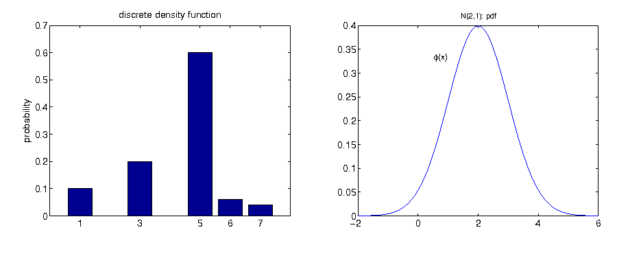
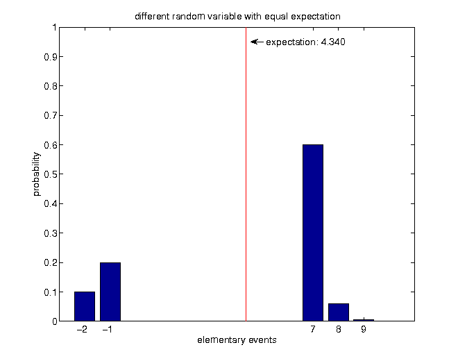
Examples
$$\begin{align*} \mathbb{E}\left[X\right] & =\sum_{i=1}^{5}x_{i}\mathbb{P}\left(X=x_{i}\right)\\ & =1\cdot0.1+3\cdot0.2+5\cdot0.6+6\cdot0.06+7\cdot0.04=4.34 \end{align*}$$
$$\begin{equation*} \mathbb{E}\left[X\right]=-2\cdot0.1-1\cdot0.2+7\cdot0.6+8\cdot0.06+9\cdot0.0067=4.34 \end{equation*}$$
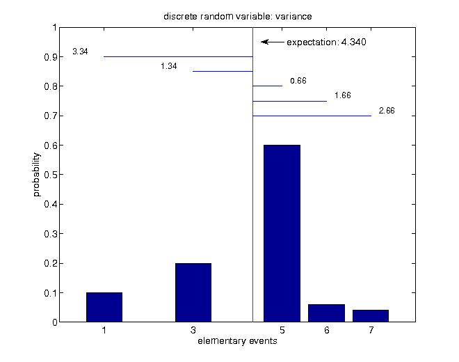
Variance
The variance provides a measure of dispersion around the mean.
Discrete random variables
The variance is defined by
$$\begin{equation*} \mathbb{V}\left[X\right]=\sigma_{X}^{2}=\sum_{i=1}^{N}\left(X_{i}-\mu_{X}\right)^{2}\mathbb{P}\left(X=x_{i}\right), \end{equation*}$$
where $\sigma_{X}=\sqrt{\mathbb{V}\left[X\right]}$ denotes the standard deviation of X.
Continuous random variables
For continuous variables, the variance is defined by
$$\begin{equation*} \mathbb{V}\left[X\right]=\sigma_{X}^{2}=\int_{-\infty}^{\infty}\left(x-\mu_{X}\right)^{2}f\left(x\right)dx \end{equation*}$$
Example
$$\begin{align*} \mathbb{V}\left[X\right] & =\sum_{i=1}^{5}\left(x_{i}-\mu\right)^{2}\mathbb{P}\left(X=x_{i}\right)\\ & =3.34^{2}\cdot0.1+1.34^{2}\cdot0.2+0.66^{2}\cdot0.6+1.66^{2}\cdot0.06+2.66^{2}\cdot0.04\\ & =2.1844\neq14.913 \end{align*}$$
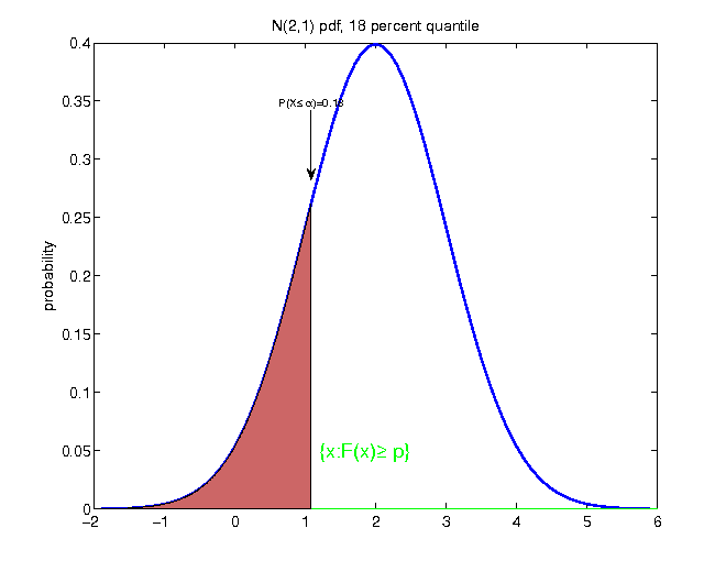
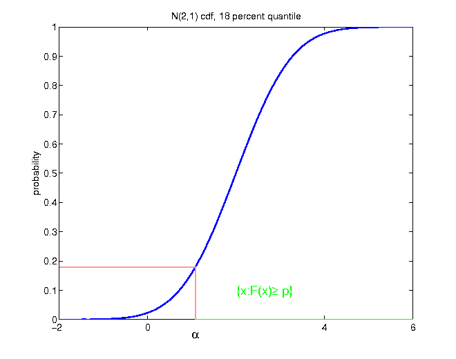
Quantiles
Quantile
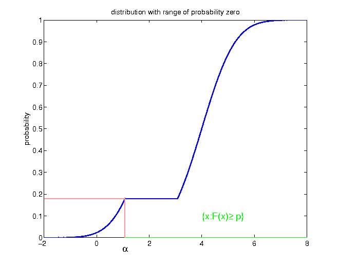
Let X be a random variable with cumulative distribution function F. For each p ∈ (0, 1), the p-quantile is defined as
$$\begin{equation*} F^{-1}\left(p\right)=\inf\left\{ x|F\left(x\right)\geq p\right\} . \end{equation*}$$
Quantile
- measure of location
- divides distribution in two parts, with exactly p * 100 percent of the probability mass of the distribution to the left in the continuous case: random draws from the given distribution F would fall p * 100 percent of the time below the p-quantile
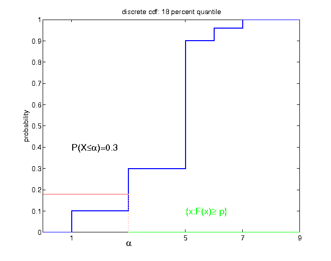
- for discrete distributions, the probability mass on the left has to be at least p * 100 percent:
$$\begin{equation*} F\left(F^{-1}\left(p\right)\right)=\mathbb{P}\left(X\leq F^{-1}\left(p\right)\right)\geq p \end{equation*}$$
Example
Example: cdf
Example
Example
Summary: information reduction
Incomplete information can occur in two ways:
- a coarse filtration
- only values of some measures of the underlying distribution are known (mean, dispersion, quantiles)
Any reduction of information implicitly induces that some formerly distinguishable distributions are undistinguishable on the basis of the limited information.
- tradeoff: reducing information for better comprehensibility / comparability, or keeping as much information as possible
General problem
Quantity of interest
$$\begin{equation*} \varrho(\bf{Z})=g(\bf{X}),\quad \bf{X}=(X_{1},\ldots, X_{d}) \end{equation*}$$
- instead of the complete distribution of Z, interest only lies in some measure $\varrho$ (expectation, variance, ...)
Updating information
opposite direction: updating information on the basis of new arriving information
concept of conditional probability
Example
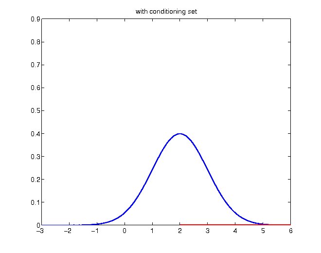
- with knowledge of the underlying distribution, the information has to be updated, given that the occurrence of some event of the filtration is known
- normal distribution with mean 2
- incorporating the knowledge of a realization greater than the mean
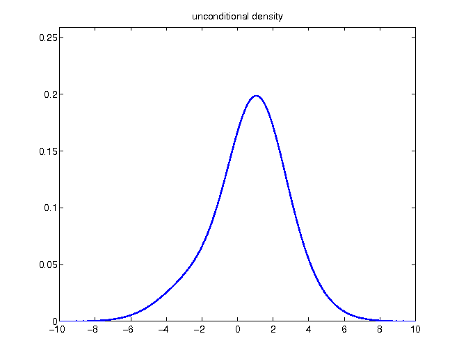
Unconditional density
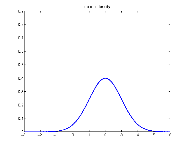
Given the knowledge of a realization higher than 2, probabilities of values below become zero:
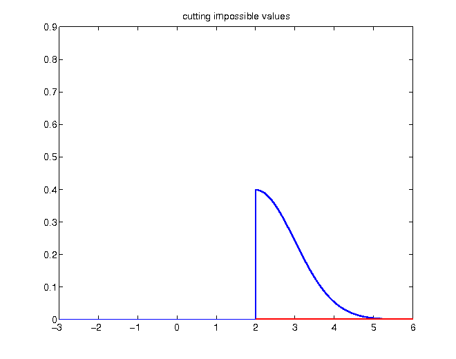
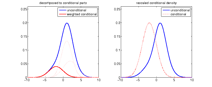
Without changing relative proportions, the density has to be rescaled in order to enclose an area of 1:
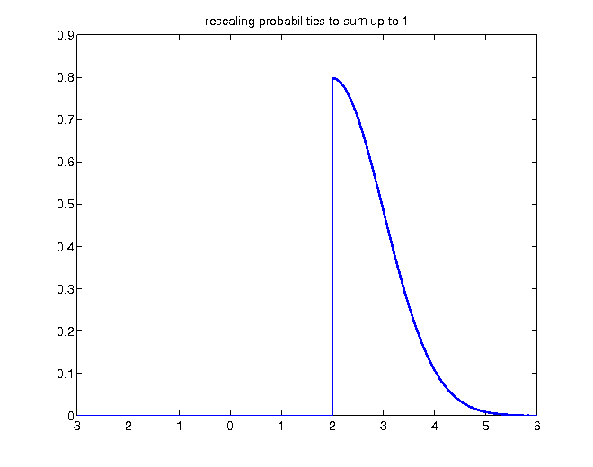
- original density function compared to updated conditional density
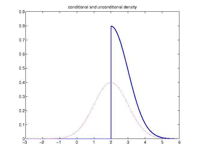
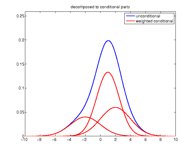
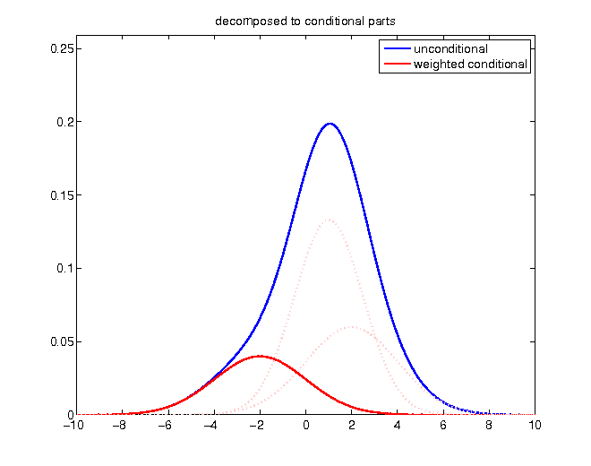
Decomposing density