Risk management
Functions applied to random variables
Christian Groll
Univariate transformations
Target
- target random variable Y: function of random variable with know distribution
$$\begin{align*} X&\sim F_{X}\\ Y&=g(X)\\ Y&\sim ? \end{align*}$$
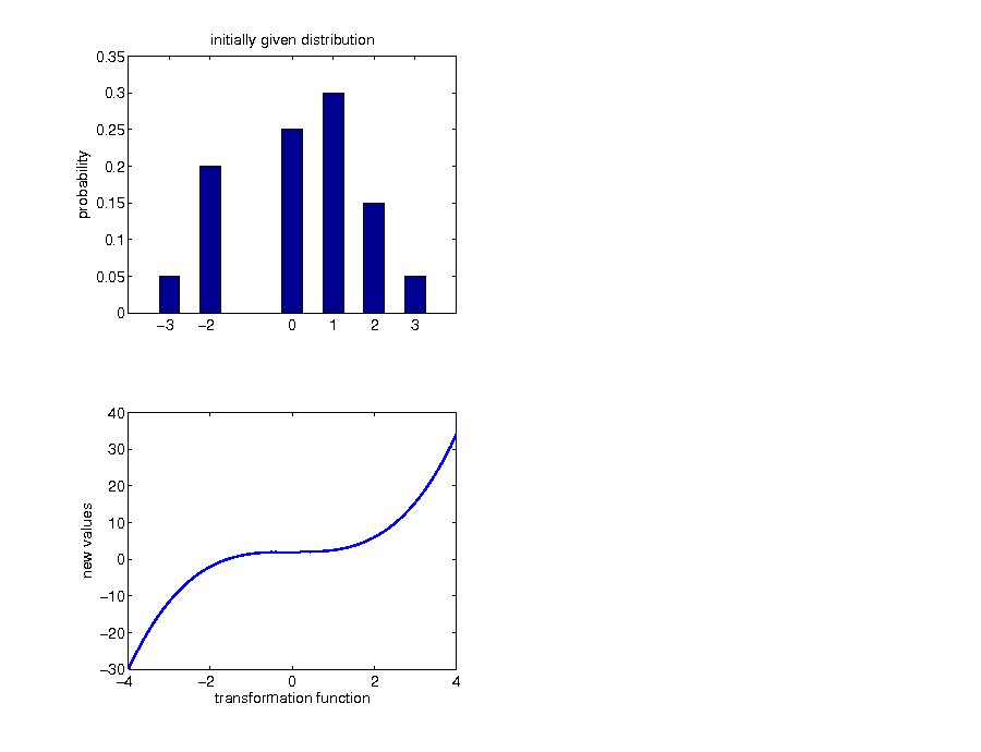
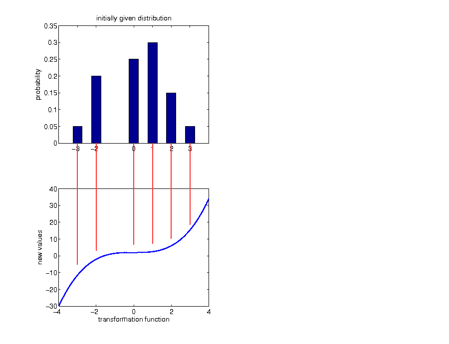
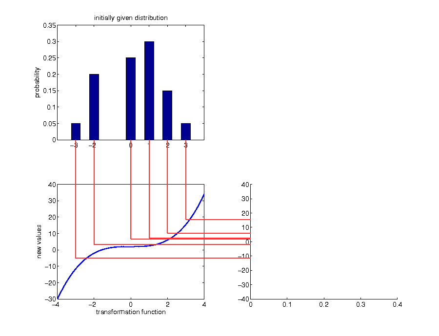
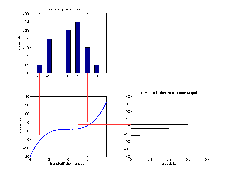
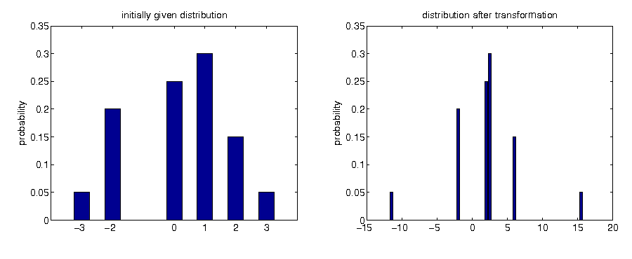
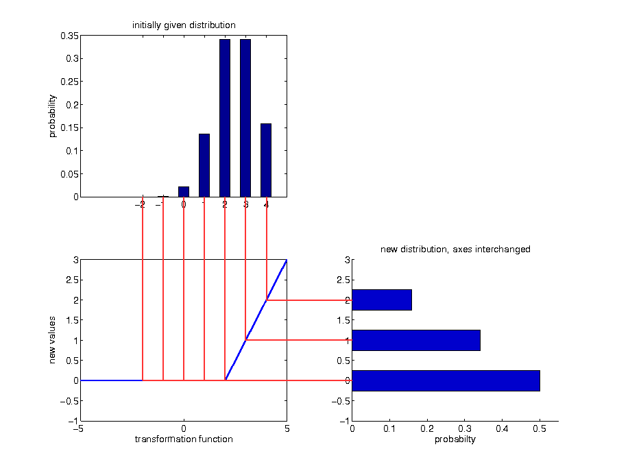
Example: discrete case
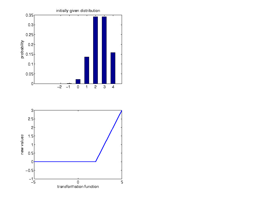
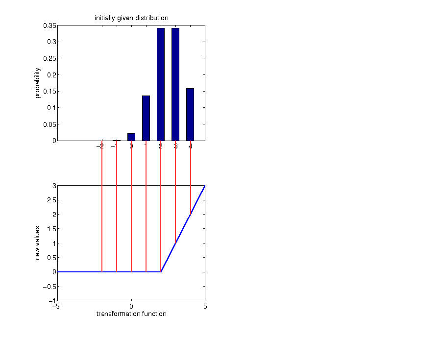
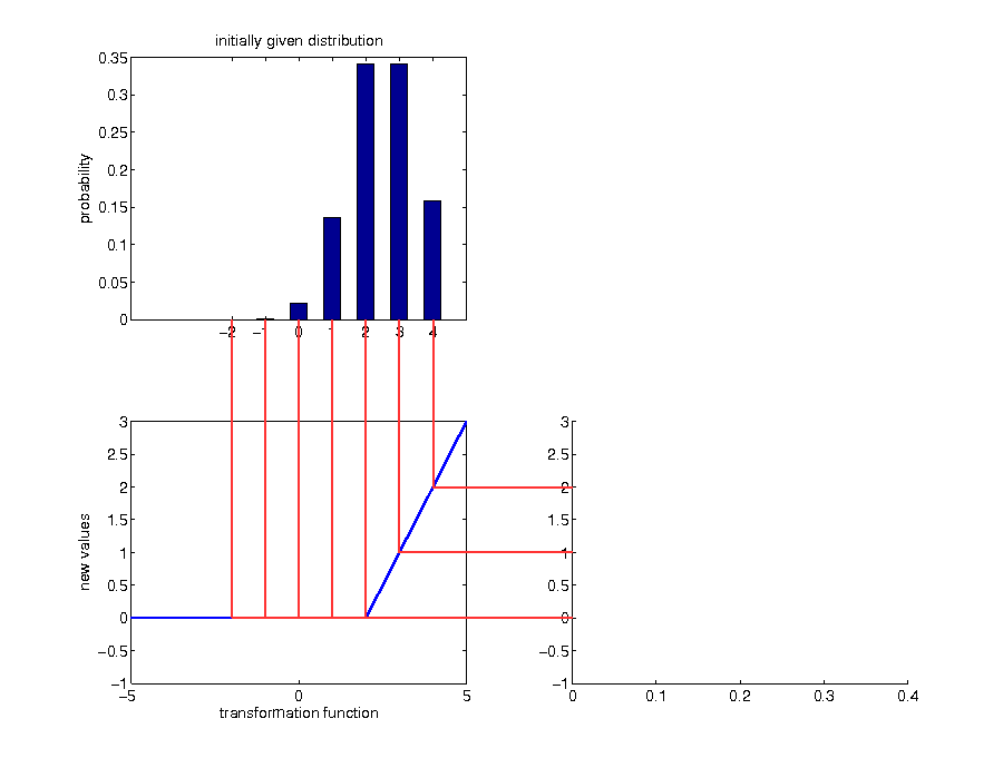
Example: call option payoff
Transformations of continuous random variables
Analytical formula
Transformation theorem
Let X be a random variable with density function f(x), and g(x) be an invertible bijective function. Then the density function of the transformed random variable Y = g(X) in any point z is given by
$$\begin{equation*} f_{Y}\left(z\right)=f_{X}\left(g^{-1}\left(z\right)\right)\cdot\left|\left(g^{-1}\right)^{'}\left(z\right)\right|. \end{equation*}$$
Problems
- given that we can calculate some measure $\varrho_{X}$ of the original random variable X, it is not ensured that $\varrho_{Y}$ can be calculated for the new random variable Y, too: e.g. if $\varrho$ envolves integration
- what about non-invertible functions?
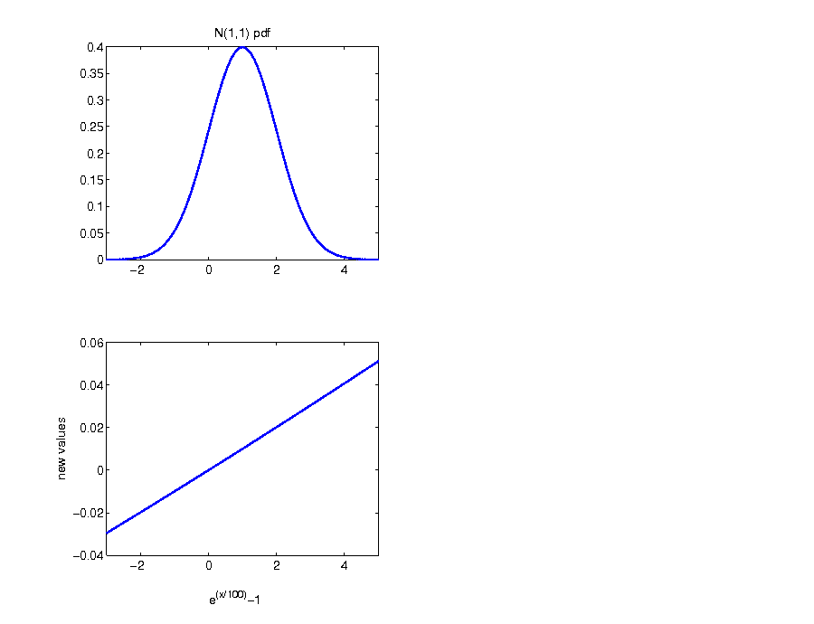
Example: return distribution
- traditional financial modeling: normally distributed logarithmic returns
- for example: percentage logarithmic returns
$$\begin{equation*} R^{\log}:=100 r^{\log} \end{equation*}$$
- net returns as function of Rlog:
$$\begin{equation*} r=\exp (R^{log}/100)-1 \end{equation*}$$
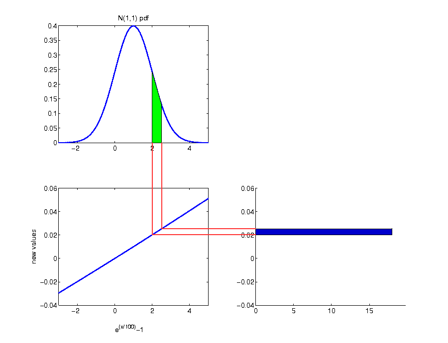
Analytical calculation
- according to the transformation theorem, we get for the distribution of net returns:
$$\begin{align*} f_{r}\left(z\right)&=f_{R^{log}}\left(g^{-1}\left(z\right)\right)\cdot\left|\left(g^{-1}\right)^{'}\left(z\right)\right|\\ g\left(x\right)&=e^{x/100}-1 \end{align*}$$
⇒ calculating each part
- calculation of g − 1 :
$$\begin{alignat*}{2} x & =e^{y/100}-1 & \,\Leftrightarrow\\ x+1 & =e^{y/100} & \,\Leftrightarrow\\ \log\left(x+1\right) & =y/100 & \,\Leftrightarrow\\ 100\cdot\log\left(x+1\right) & =y \end{alignat*}$$
- calculation of (g − 1)′:
$$\begin{equation*} \left(100\cdot\log\left(x+1\right)\right)^{'}=100\cdot\frac{1}{x+1} \end{equation*}$$
- plugging in leads to:
$$\begin{equation*} f_{r}\left(z\right)=f_{R^{log}}\left(100\cdot\log\left(z+1\right)\right)\cdot\left|\frac{100}{z+1}\right| \end{equation*}$$
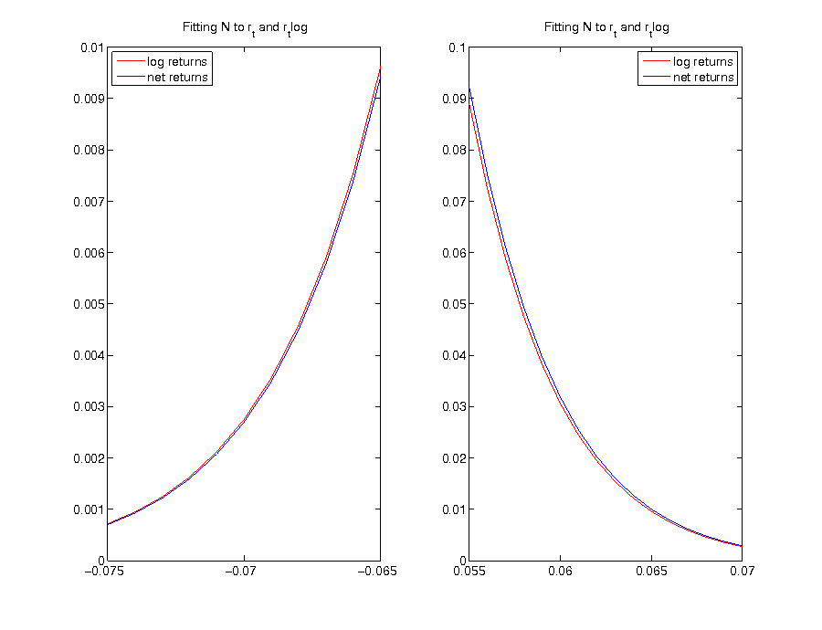
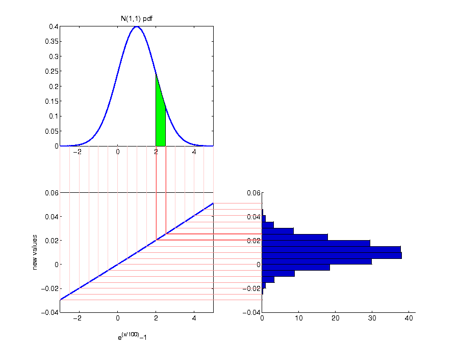
- although only visable under magnification, there is a difference between a normal distribution which is directly fitted to net returns and the distribution which arises for net returns by fitting a normal distribution to logarithmic returns
- the resulting distribution from fitting a normal distribution to logarithmic returns assigns more probability to extreme negative returns as well as less probability to extreme positive returns
Example: inverse normal distribution
- application of an inverse normal cumulative distribution as transformation function to a uniformly distributed random variable
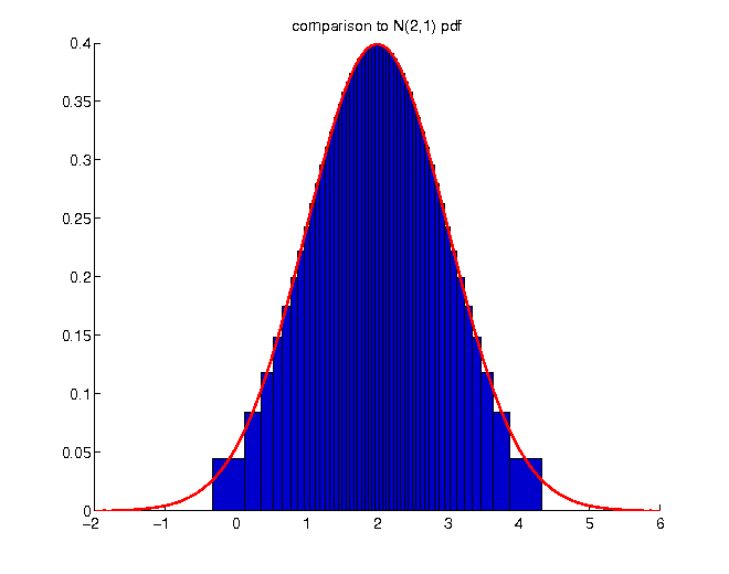
- the resulting distribution really is the normal distribution
- application of an inverse cdf to a uniformly distributed random variable forms the basis of Monte Carlo simulation
Monte Carlo simulation
Let X be a univariate random variable with distribution function FX. Let FX − 1 be the quantile function of FX, i.e.
$$\begin{equation*} F_{X}^{-1}\left(p\right)=\inf\left\{ x|F_{X}\left(x\right)\geq p\right\} ,\quad p\in\left(0,1\right). \end{equation*}$$
Then, we can simulate random variables with arbitrary distribution function FX through:
$$\begin{equation*} F_{X}^{-1}\left(U\right)\sim F_{X},\quad \text{for } U\sim\mathbb{U}\left[0,1\right] \end{equation*}$$
Proof
Let X be a continuous random variable with cumulative distribution function FX, and let Y denote the transformed random variable Y := FX − 1(U). Then
$$\begin{equation*} F_{Y}\left(x\right)=\mathbb{P}\left(Y\leq x\right)=\mathbb{P}\left(F_{X}^{-1}\left(U\right)\leq x\right)=\mathbb{P}\left(U\leq F_{X}\left(x\right)\right)=F_{X}\left(x\right) \end{equation*}$$
so that Y has the same distribution function as X.
- the reverse direction also is important:
Probability integral transformation
If FX is continuous, then the random variable FX(X) is standard uniformly distributed, i.e.
$$\begin{equation*} F_{X}(X)\sim \mathbb{U}([0,1]) \end{equation*}$$
and is called probability integral transform.
Proof
$$\begin{align*} \mathbb{P}(F_{X}(X)\leq u)&=\mathbb{P}(X\leq F^{-1}_{X}(u))\\ &=F_{X}(F_{X}^{-1}(u))\\ &=u \end{align*}$$
$$\begin{equation*} \Rightarrow\quad \mathbb{P}(F_{X}(X)\leq u)=\mathbb{P}(U\leq u) \quad U\sim \mathbb{U}([0,1]) \end{equation*}$$
Linear transformations
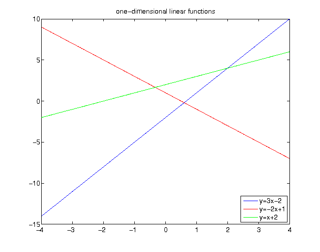
- linear transformation functions are given by
$$\begin{equation*} g(x)=ax+b \end{equation*}$$
examples of linear functions:
Analytical solution
- calculate inverse g − 1 :
$$\begin{equation*} x=ay+b\,\Leftrightarrow\, x-b=ay\,\Leftrightarrow\frac{x}{a}-\frac{b}{a}=y \end{equation*}$$
- calculate derivative (g − 1)′ :
$$\begin{equation*} \left(\frac{x}{a}-\frac{b}{a}\right)^{'}=\frac{1}{a} \end{equation*}$$
- putting parts together:
$$\begin{align*} f_{g\left(X\right)}\left(z\right) & =f_{X}\left(g^{-1}\left(z\right)\right)\cdot\left|\left(g^{-1}\right)^{'}\right|=f_{X}\left(\frac{z}{a}-\frac{b}{a}\right)\cdot\left|\frac{1}{a}\right| \end{align*}$$
- interpretation: shifting b units to the right, stretching by factor a
Linear transformation: expectation
- stretching and shifting also is transferred to the expectation of a linearly transformed random variable Y := aX + b:
$$\begin{equation*} \mathbb{E}\left[Y\right]=\mathbb{E}\left[aX+b\right]=a\mathbb{E}\left[X\right]+b \end{equation*}$$
Linear transformation: variance
$$\begin{align*} \mathbb{V}\left[Y\right]&=\mathbb{E}\left[\left(Y-\mathbb{E}\left[Y\right]\right)^{2}\right]\\ & =\mathbb{E}\left[\left(aX+b-\mathbb{E}\left[aX+b\right]\right)^{2}\right]\\ & =\mathbb{E}\left[\left(aX+b-a\mathbb{E}\left[X\right]-b\right)^{2}\right]\\ & =\mathbb{E}\left[\left(a\left(X-\mathbb{E}\left[X\right]\right)+b-b\right)^{2}\right]\\ & =a^{2}\mathbb{E}\left[\left(X-\mathbb{E}\left[X\right]\right)^{2}\right]\\ & =a^{2}\mathbb{V}\left[X\right] \end{align*}$$
Remarks
- calculation of mean and variance of a linearly transformed variable neither requires detailed information about the distribution of the original random variable, nor about the distribution of the transformed random variable
- knowledge of the respective values of the original distribution is sufficient
- for non-linear transformations, such simple formulas do not exist
- most situations require simulation of the transformed random variable and subsequent calculation of the sample value of a given measure